Let's Create a Tree from Scratch
When we learned linear regression we learned the underlying model by looking at the equation. However, decision trees are not based on a mathematical equation. Instead, they are based on a series of conditions, so to understand how they work let's make one from scratch! We will explore the code that underlies decision trees, visualize the current step using a subset of the iris dataset, and then put this code into functions, so that we can pull it all together into our very own decision tree function.
Let's start by providing the same decision tree image we saw in the previous lesson, as we will be referencing it throughout this lesson.
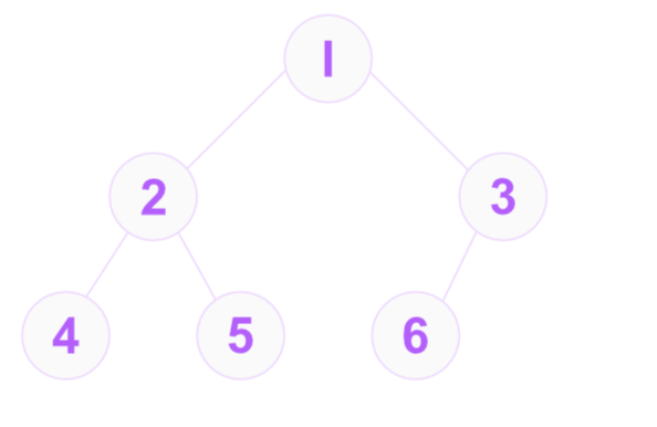
And we will use the following subset of the iris dataset to visualize the decision tree as we build it.
| Sepal.Length | Petal.Length |
|---|---|
| 5.1 | 1.4 |
| 4.9 | 1.4 |
| 4.7 | 1.3 |
| 6.3 | 6 |
| 5.8 | 5.1 |
Creating nodes using classes
To begin, we need to consider, how will we store the information regarding the decision tree's nodes. In this application we will use a class to store the information for each node. The benefit of this is that it collects the information into one place, and allows us to create multiple instances of the class, each representing a different node.
We make a distinction of two types of nodes. Any node that has children - nodes connected to it below it, such as nodes: 1, 2, and 3 in the image - are called decision nodes. Nodes that have no children - nodes: 4, 5, and 6 - are called leaf nodes. So we'll construct these as two different classes. Let's go over the details of each class and map it to the code that constructs these in the below code editor.
- Node: We will want to apply types to our classes and functions, so we will create a Node class that will be the union of the DecisionNode and LeafNode class types. Meaning any variable that is of type Node can be either a DecisionNode or a LeafNode.
- DecisionNode: Has three parameters split, left,
and right, which are saved to the class as attributes.
- split: This is the value that the decision node will use to split the
data on. The datatype is float, which means it can be any number. A split is
a condition such as
if x ≤ 5, where 5 is the split value. - left: This is the node that the decision node will send the data to if the data is less than the split value, in the above example any x-values less than or equal to five. The datatype is Node, which is a union of the DecisionNode and LeafNode class types.
- right: This is the node that the decision node will send the data to if the data is greater than the split value, in the above example any x-values greater than five. The datatype is also Node.
- split: This is the value that the decision node will use to split the
data on. The datatype is float, which means it can be any number. A split is
a condition such as
- LeafNode: Has one parameter value, which is saved to the class as an attribute. The value is the predicted value of the dependent variable for the data that falls within the leaf node. And the datatype is float.
Considering splits
Let's start making the decision tree by hand. In this application we will begin by choosing the split values, but later we will write a function that will choose the split values for us.
We will start by creating the root node, which is node 1 in the image above. The root node is a decision node, so we will create an instance of the DecisionNode class. We set the split value to 5. When we set the split value to 5, we are splitting the data based on the variable with values below or above it. In this particular instance, two rows - which we will call observations from now on - will go to the left node, and three observations will go to the right node.
Left data that goes to node 2
| Sepal.Length | Petal.Length |
|---|---|
| 4.9 | 1.4 |
| 4.7 | 1.3 |
Right data that goes to node 3
| Sepal.Length | Petal.Length |
|---|---|
| 5.1 | 1.4 |
| 6.3 | 6 |
| 5.8 | 5.1 |
The predicted value for either node is the average of the
outcome variable, which is petal length. So for node 2
this is:
We could continue with this until we reach the maximum depth of the tree, but let's stop here for now. We will want to generalize this process to find the best split value for us. But to determine what is the best split value, we need to choose a model evaluation metric, which will be the topic of the next section.
A model evaluation metric
A model evaluation metric is a quantifiable measure used to assess the performance of a model, enabling comparison with other models. In this application we will choose the mean squared error (mse) as our model evaluation metric. The mean squared error is the average of the squared differences between the predicted value and the actual value. But in this case we will modify it to be the average of the squared differences between the outcome values in each node and the mean of these values. This is so we can save the task of prediction to the next lesson.
Let's write a function that will calculate the mean squared error
for us. We will call this function calculate_mse. It will take one
parameter, a numpy array of values, and return the mean squared
error.
Finding the best split
Now that we have a model evaluation metric, we can write a function
that will find the best split value for us. We will call this function
find_best_split. Let's go over the code.
- X: A numpy array of feature values to split on.
- y: A numpy array of outcome values.
- Lines 2 and 3: Initialize the best split value and its associated mse for comparison later.
- Line 4: Loop through each unique value in the feature array.
- Lines 5 and 6: Split the data into two groups, values less than or equal to the split value will be put into the variable called left_mask, and remaining in the variable right_mask.
- Lines 7, 8, and 9: Calculate the mean squared error for each group and sum them together.
- Lines 11, 12, and 13: Check if the current total_mse is less than the previous best min_mse (a smaller mse is better). Since we start with the best mse as infinity, this will always be true for the first value. And whenever this condition is is true, then we update both the min_mse and the best_split value.
- Line 15: Return the best split value and its associated minimum MSE. These are written here with a comma, which means they will be returned as a tuple.
- Line 17: Call the function with our iris data, and destructure the returned tuple into two variables, best_split and min_mse.
Building the tree
Now that we have a function that will find the best split value for us,
we can write a function that will build the tree for us. We will call
this function build_tree. Note that this function is a
type of function called a recursive function. These are a class
of functions that call themselves. They are usually more difficult to understand
than normal functions. So if you would care to learn about them or have some review
on it, then feel free to check out these two lessons on recurions:
Learn recursion's base case
and Learn recursion by studying
path walking on trees. Once you are comfortable with recursion then let's
go over the code.
- X: A numpy array of feature values to split on and a.
- y: A numpy array of outcome values.
- depth: The current depth of the tree.
- max_depth: The maximum depth of the tree.
- Lines 2 and 3: Check if the current depth is equal to the maximum depth. Or if the number of unique values in the outcome array is equal to one. If either of these conditions are true, then we return from the function creating a leaf node with it's value equal to the mean of the outcome values passed into it.
- Line 5: Call the
best_splitfunction and get the split and mse values. - Lines 6 and 7: If the mse is infinity, then that means there is no split value that will improve the model. So we would again return from the function creating a leaf node with it's value equal to the mean of the outcome values.
- Lines 9 and 10: Split the data into two groups.
- Lines 11 and 12: Recursively call this function on the left and right data, and increment the depth by one to continue the tree building process. This will continue until the depth is equal to the maximum depth or the number of unique values in the outcome array is equal to one in either case causing one of the if conditions to be true leading to the function returning a leaf node and ending the recursion.
- Line 19: Run the function on our iris data with a maximum depth of 1, meaning the tree will only have one decision node and two leaf nodes.
Concluding thoughts
We have now created a decision tree from scratch! We have learned how to create nodes using classes, how to find the best split value, and how to build the tree. Feel free to play around with the code and try larger depths to see how the tree changes. This is a simplified tree building process, but it is the foundation for the more complex kind of tree that is used in the scikit-learn library.