Let's begin our journey into linear regression by first understanding what it is, and why it is so important in data science.

Linear regression is a statistical method used to model the relationship between two or more variables. It is a very simple, yet powerful, method that is used in many different fields. In data science, it is used to understand the relationship between variables in a dataset, and to predict the value of a variable given the value of another variable.

Let's take a look at a simple example using the iris dataset. We will use the sepal length and petal length variables to illustrate the concept of linear regression. In this example, we will use sepal length as the independent variable, also known as the explanatory variable or feature; this is the variable that we assume influences or predicts the dependent variable, which is the variable of interest. We will use petal length as the dependent variable, also known as the response variable, outcome variable, or target. Due to how much linear regression is used in a variety of fields there are many different terms that refer to the same thing, so one challenge starting out is just becoming familiar with the terminology that is more common in your field of interest.

Let's take a look at the plot of these two variables with the best fit line added in (the black line in the plot below). The best fit line is the line that minimizes the distance between all the points in the plot. We will discuss how to calculate this line shortly.

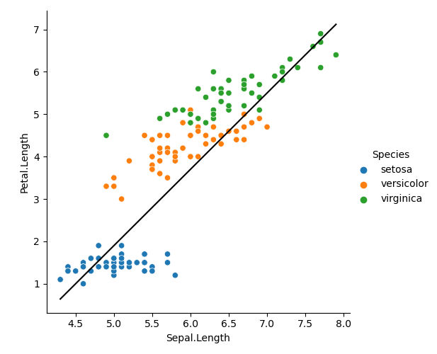
We can see that there is a clear relationship between the two variables, and that the best fit line does a good job of capturing this relationship. We can also see that the best fit line is not perfect, and that there is some variation in the data. This variation is due to the fact that there may be either other variables that influence petal length that we are not accounting for in this model, or that additional complexity between the two variables exists that we are not capturing with a straight line. Next, let's go over the the equation for this line, before concluding with going over the code that produced this plot.

Equation of a line

The linear regression model is the following equation:

y = mx + b + \varepsilon

Let's go over what each of these variables mean in the next few sections.

The dependent variable: y

The dependent variable is the variable that we want to learn more about. In our example, this is the petal length variable. In the equation, it is represented by the variable y. It is called the dependent variable because it represents the outcome or effect that we are trying to predict or explain. It is presumed to depend on or be influenced by the independent variable. This means that changes in sepal length are hypothesized to cause changes in petal length.

The independent variable: x

The independent variable is the variable that we hypothesize influences the dependent variable. In our case, sepal length and represented in the equation as x. It is called the independent variable because it is presumed to be independent of the dependent variable. This means that there is a one-way direction of influence from the independent variable to the dependent variable, but not in the reverse direction. This is important to note because it underscores the causal assumption in our analysis - we are investigating how changes in sepal length might affect petal length, not vice versa. Understanding this directional relationship starts with you, the data scientist, in how you choose to formulate a hypotheses.

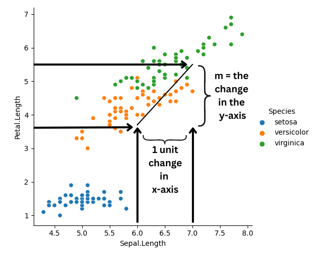
The slope: m

The slope, represented by m, is the rate of change of the dependent variable with respect to the independent variable. In simpler terms, it is the amount that petal length changes for every unit change in sepal length. The slope tells us the relationship between the two variables. If the slope is positive, then the two variables are positively related, meaning that as sepal length increases, so is petal length expected to increase. And vice-versa if the slope is negative.

For example, let's look at the plot below. The slope is positive, with m = 0.5. We put a black line from the x-axis at sepal length = 6 to sepal length = 7. Since the difference between 7 and 6 is 1, we call this a unit change. We can see that the difference between petal length at these two endpoints is is roughly 5.5 - 3.5 = 2, which is close to the the slope we calculated earlier at 1.8.

The intercept: b

The intercept, represented by b, is the value of the dependent variable when the independent variable is equal to zero. In our example, this is not a very meaningful value, since sepal length cannot be equal to zero. However it is still necessary to include in the equation so that the line we estimate closely overlaps with the data.

The error: \varepsilon

The error, represented by \varepsilon, is the difference between the actual value of the dependent variable, y, and the predicted value of the dependent variable, \hat{y}. The error is also known as the residual. The residual is the final piece to the equation. It captures the fact that there are other variables that influence the dependent variable that we are not accounting for in our model. It is also the reason why the best fit line is not perfect, and why there are points above and below the estimated line.

The code that produced the plot

To conclude this lesson let's go over the code line-by-line that produced the plot. Note that the libraries we imported are hidden in the code below, if you want to see what they are, check out the Code environment drop-down menu at the top of the page.

• Line 2: This plots the iris dataset with sepal length on the x-axis and petal length on the y-axis.
• Lines 5 & 6: We will see in the next lesson how to calculate these. For now, just know that these are the values of the slope and intercept.
• Line 9: To formulate this in the same way as the equation we create the x variable.
• Line 12: We use the slope, intercept and x to calculate the predicted \hat{y} (y_hat values) for the best fit line.
• Lines 15: We add the best fit line to the plot. We use the sns.lineplot along with the ax argument to add the line to the existing plot specifying the plot with the plot.ax value.