Knowing what the complexity of a program is valuable information. However figuring it out for every function one writes may be exhausting. That is why researchers seek to find generalized solutions to certain types of problems. Functions with recursion are particularly interwoven and its hard to untangle their full complexity. In this lesson we will learn how, given a specific form of recursion algorithm - known as divide and conquer algorithms, we may know its complexity without having to know their full intricacies.

This will likely be the most difficult topic in this course. This lesson requires a greater amount of mathematical maturity than the rest of the course. Try and read as much of it as you can, but don't feel discouraged if the topics aren't sticking and wish to move on to something more tangible.

When we state and solve recurrences, we will omit floor, ceiling, and boundary conditions. This is because they have negligible effect on the actual complexity of the algorithm. We might get a floor or ceiling effect when n is not a power of b. However it's been shown that including these won't actually change the boundary conditions and so to simplify the solution a little bit, we will ignore it. If you wish to learn more about it, or any other part of the master theorem, please refer to the excellent textbook Introduction to algorithms 3rd edition by Leiserson, Rivest, and Stein.

We will separate this lesson into two parts. First, a definition of the theorem and its specific cases. Second, how a recursion tree might be used to prove the master theorem.

Definition

The master theorem solves recurrences of the form below.

Where a and b are constants, T might be considered total time, n is the size of the input, and f is a function.

This recurrence defines the run time of algorithms that divides a problem of size n into a subproblems, each of size n/b. f(n) includes the cost of dividing the problem and the cost of combining the results of the subproblems.

the master theorem provides bounds on T(n) under three different scenarios.

if f(n)=	Bound on T(n)	Constraints
1. f(n) = O(n^{log_{b}{a}-\epsilon})	\Theta(n^{log_{b}{a}})	\epsilon > 0
2. f(n) = \Theta(n^{log_{b}{a}})	\Theta(n^{log_{b}{a}}lg{n})
3. f(n) = \Omega(n^{log_{b}{a}+\epsilon})	\Theta(f(n))	\epsilon > 0, af(n/b) \leq cf(n), c < 1

Example

Given the recurrence relations below, we will use the master theorem to quickly solve a tight bound on it. In the next section we will verify this using recursion trees.

We see a=2, b=2, f(n) = n. Now we need to choose which of the three scenarios provides a bound on f(n). For completeness, we will do all three. We will ignore the bound symbol and only do the computation inside of it. Once we find the right scenario then we will include the bound symbol.

1. n^{log_{2}{2}-1} = n^0 = 1, here we use \epsilon = 1 for simplicity, we could use a smaller float, but it will not change the result. Since this is too small to bound f(n), it is not this scenario.

2. n^{log_{2}{2}} = n^1 = n. Since n \leq n, this looks like a good bound. Next, we can plug in our variables to get a bound for T: n^{log_{2}{2}} lg({n}) = n lg({n}), giving us a final bound of \Theta(n lg({n})).

3. n^{log_{2}{2}+1} = n^2. While this also bounds f(n), we have already found a tighter bound.

This recurrence relation is actually one for mergesort. We will provide a bound on mergesort in three different ways, using the master theorem as we just did, below using a recursion tree, and third using line-by-line code in the mergesort lesson.

Recurrence tree

We've been using bounds from the master theorem without any motivation as to where they came from. In this section we will attempt to elucidate an answer.

We will start by drawing a recursion tree for T(n) = 2 T(n/2) + n.

A recursion tree is a tree where each node represents the cost of a single subproblem.

We can find the total cost for a recursion relation by summing its corresponding recursion tree. This total cost may then be used to define a bound.

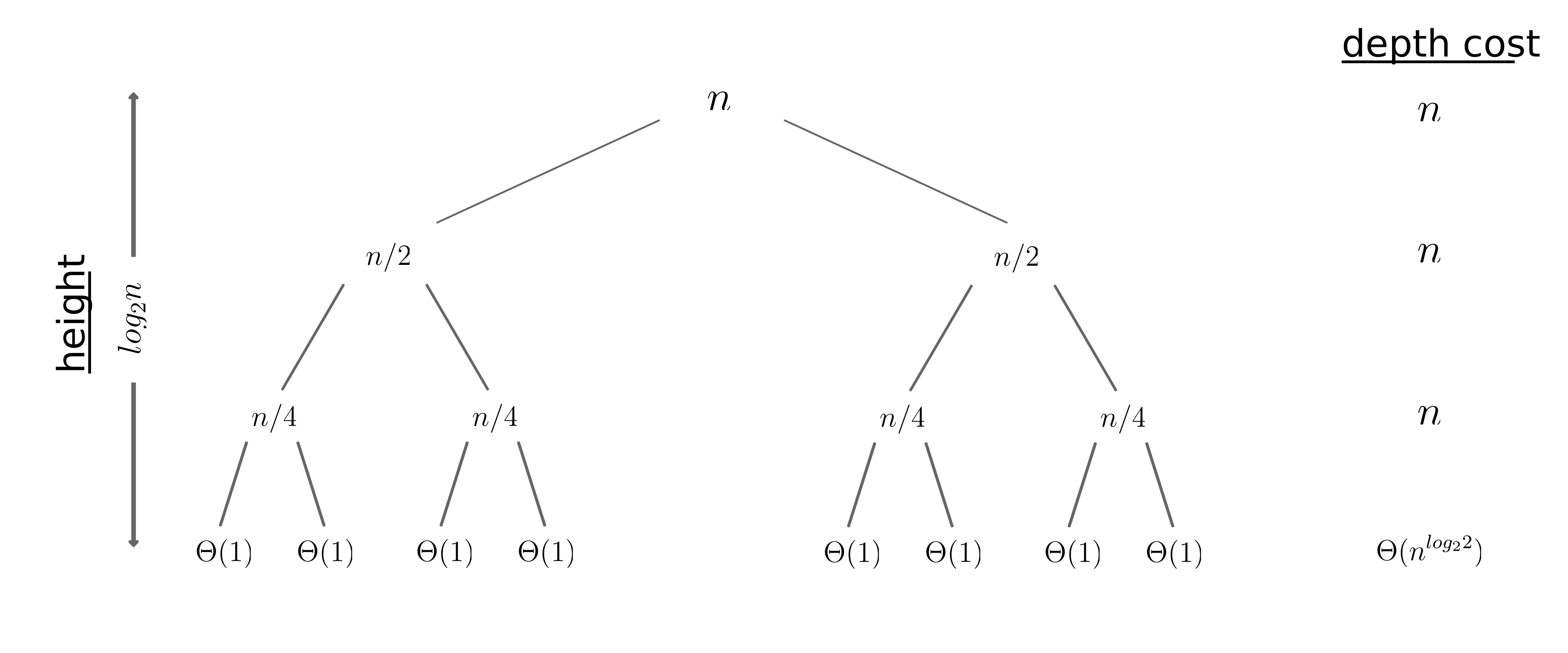
The root has initial cost n with two children, each with cost n/2. These two children similarly have two children each, where their cost is n/4. To find the cost at any given depth, we sum across that depth. So the cost at depth one is n/2 + n/2 = n and at depth two is 4 * n/4 = n and so on.

We can make some observations from this tree. First, the height is log_2{n}. Note, log_2{n} is equivalent to lg(n) since it's used frequently. Second, the cost at any depth sans leaf nodes is n. Third, the cost for the leaf nodes is \Theta(n) (It's actually \Theta(n^{log_{2}{2}}), however log_{2}{2}=1).

The following equation represents the total cost for this recursion tree.

The 2^i in the numerator is the total number of nodes at depth i, while 2^i in the denominator is the fraction we see in the tree as the amount of work is reduced. These terms cancel each other out.

The summation of a constant is simply a product of the constant and the upper summation term.

We may now take an upper bound of this equation; also, O(\Theta(n)) = O(n).

Great! We reached the same conclusion as the master theorem provided us. This was just one recurrence tree, what about others? We may write a generalized recursion tree for any equation that is solved by the master theorem as below.

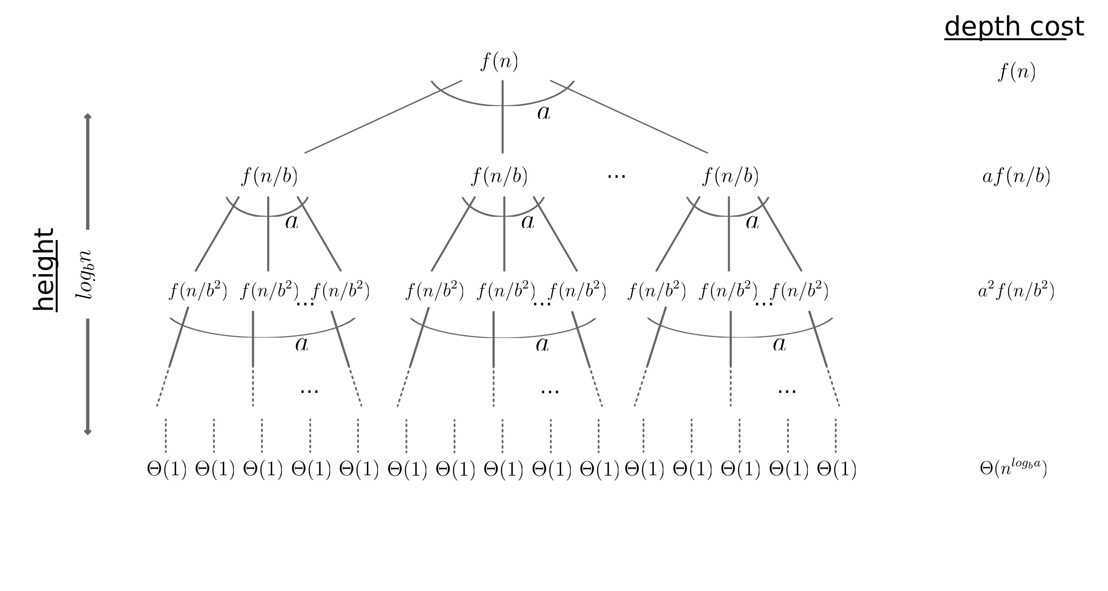
Summing every node except the leaves, then including the leaves gives the equation below.

The summation represents the cost of dividing the problem into subproblems and then recombining them. The cost of the leaves is the cost for the base case at the end of recursion.

The master theorem may be seen to handle three cases in a recursion tree. 1) When the work is dominated by the leaves. 2) When the work is equally distributed among the levels of the tree. 3) When the work is dominated by the root.

The last step is to find a bound for this generalized equation for each of the three scenarios. However the proof is even more rigorous than anything previous and is outside the scope of this course. If one really wishes to learn about it, please refer to chapter 4.6.1 in Introduction to algorithms 3rd edition.

Practice exercise 01

Use the master theorem to provide a bound on the recurrence relation 9T(n/3) + n.

show solution

Practice exercise 02

Use the master theorem to provide a bound on the recurrence relation 3T(n/3) + n^2.

show solution